Rotor Systems: Analysis and Identification
(Errata and Answers to Selected Exercise
Problems)
Errata in “Rotor Systems: Analysis and Identification, CC Press,
Boca Raton, USA” Authored Rajiv Tiwari
(please report if you
find more: rtiwari@iitg.ac.in)
|
S.N. |
Page |
Specific location |
Correction/inclusion |
|
|||
|
Preface |
xvii |
List of Ph D students helped |
Rajeswara Rao Bhyri |
✔ |
|||
|
|
|
|
|
|
|||
|
Ch02 |
22 |
Section 2.1 |
“p” is missing In I = p d4/64 |
✔ |
|||
|
|
31 |
Example 2.1 |
of |
|
|||
|
|
40 |
|
Herein, the moment is taken with respect to the C, the
moment can also be taken about G. In that case moment equation will contain x
and y along with theta. But since Eqns. (a) and (b) contain theta we need to
solve all three equations simultaneously. In chapter 11 the moment was taken
about the G to get EOM in theta direction (page 671, Eqn. c). |
|
|||
|
|
49 |
2.5 |
The angle, f, represents the phase between the force and the radial
response. Add “The initial phase of the unbalance is considered
as zero.” |
|
|||
|
|
69 |
Exercise 2.1 |
Show that it occurs always at frequency ratio of less than one. |
✔ |
|||
|
|
76 |
Exercise 2.25xx |
For a cantilever shaft with a thin disc at the
free end, if the transverse and torsional natural frequencies are the same,
then the ratio of the length of the shaft to the diameter of the disc would
be (take Poisson’s ratio as 1/3 for the
shaft material) (a) |
|
|||
|
|
|
|
|
|
|||
|
Ch04 |
162 |
Equation 4.52 |
|
✔ |
|||
|
|
178-179 |
Exercise 4.8 |
All jz should be jx. |
|
|||
|
|
182 |
Exercise 4.20 |
|
|
|||
|
|
|
|
|
|
|||
|
Ch05 |
204 |
Eqn. 5.5 |
Only negative sign is valid for negative m . |
|
|||
|
|
216 |
Fig. 5.29 |
In the figure |
|
|||
|
|
240 |
Exercise 5.4 |
‘+”
is missing after |
✔ |
|||
|
|
240 |
Exercise 5.5 |
Change initial tilt j to j0. |
|
|||
|
|
240 |
Exercise 5.6 |
“supported freely” to
be replaced by “simply supported” Delete whole last line “For
the cylinder .” |
|
|||
|
|
241 |
Exercise 5.7 |
A shaft of total length l
on the end bearings carries
|
|
|||
|
|
241 |
Exercise 5.8 |
kt
= 2000 N-m/ rad |
✔ |
|||
|
|
241 |
Exercise 5.8 |
Exercise 5.8 Obtain the
forward and backward transverse critical speeds of the rotor system shown
in Figure 5.48. Take the shaft as rigid. It is assumed that it
oscillates (processes) about its centre of gravity while whirling (i.e., pure
tilting without translational motion). The effective torsional stiffness of
the bearings is N-m/rad, the polar and diametral mass
moment of inertia of the rotor are 0.03 kg-m2 and 0.2 kg-m2, respectively. Consider the gyroscopic
effects. Delete last two but one lines? Not required? |
|
|||
|
|
241 |
Exercise 5.8 |
Delete the following sentence :Bearing support distance is 1 m and center of gravity of the rotor is 30 cm from the right support bearing.” |
✔ |
|||
|
|
242 |
Exercise 5.13 |
1. Add at the end of first line “of a cantilever rotor
system” 2. |
|
|||
|
|
242 |
Exercise 5.14 |
“The
|
|
|||
|
|
243 |
Exercise 5.18 |
Fig.
5.51: change shaft lengths a and b instead
of l and 2l. |
|
|||
|
|
244 |
Exercise 5.23 |
In seventh line “Ip = 0.1 kg-m2” |
|
|||
|
|
244 |
Exercise 5.24 |
Remove damping matrix:
|
|
|||
|
|
245 |
Exercise 5.29 |
“Obtain the forward and backward transverse critical speeds corresponding …” |
|
|||
|
|
246 |
Exercise 5.30 |
Change: kb = 1 kN/...k = 10 kN/m |
|
|||
|
|
247 |
Exercise 5.33 |
|
|
|||
|
|
249 |
Exercise 5.35xviii |
Then first forward natural frequency as compared to without gyroscopic effect would |
|
|||
|
|
|
|
|
|
|||
|
Ch06 |
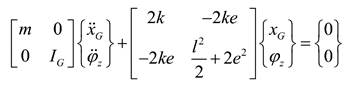
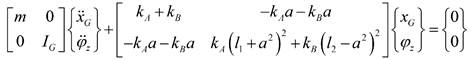
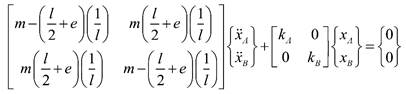
293 |
Eqn. (i) |
Correct the first row second column as:
|
|
|||
|
|
327 |
Exercise 6.10 |
(Shaft A and arm have opposite motion) |
|
|||
|
|
328 |
Exercise 6.11 |
…are
(change
is in second part |
|
|||
|
|
329 |
Exercise 6.17 |
“cm” missing in the end “16 cm” |
|
|||
|
|
331 |
Exercise 6.21 |
Delete:
IpF
= 0.006 kg-m2. |
|
|||
|
|
331 |
Exercise 6.21 |
Units “kg-m2“ missing in second and
third lines for Ip |
|
|||
|
|
332 |
Exercise 6.25 |
Given data (assumed) and from it we have
|
|
|||
|
|
|
|
|
|
|||
|
Ch07 |
352 |
Eqn. (h) |
(page322.pdf file attached) |
|
|||
|
|
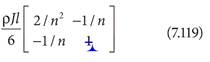
360 |
Equation 7.99 |
|
✔ |
|||
|
|
374 |
subscripts |
|
|
|||
|
|
375 |
|
write ‘2’ in second diagonal term instead of 1
|
|
|||
|
|
377 |
Example 7.8 |
Eqns. (c)
and (d): in extreme right vector “n”
to be replaced by “2”.
Also in line below Eqn. (d). |
|
|||
|
|
378 |
Example 7.8 |
Make changes
|
|
|||
|
|
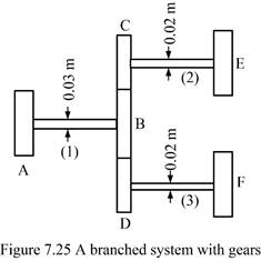
378 |
Example 7.9 |
Figure
7.25 need to be replace (its diameters are dAB = 0.03 m, dCE
= 0.02 m, and dDF = 0.02 m.)
|
|
|||
|
|
384 |
Exercise 7.9 |
Add “Speed of shaft A is 600 rpm and of the arm is 300 rpm with opposite sense of rotation.” |
|
|||
|
|
384 |
Exercise 7.10 |
|
|
|||
|
|
385 |
Example 7.12: last line |
|
|
|||
|
|
|
|
|
|
|||
|
Ch08 |
400 |
Example 8.3 |
Table 8.1 shows the systematic calculation of influence
coefficients for above expressions. Influence coefficients have been obtained
by substituting l1 = 0.05 m and l2
= 0.075 m in above expressions.
Delete 3rd and 4th columns |
|
|||
|
|
402 |
Example 8.4 |
Line 3: H4 should
be D4 |
|
|||
|
|
408 |
Eqn. 8-37 |
[F*] |
|
|||
|
|
447 |
Terms missing |
|
|
|||
|
|
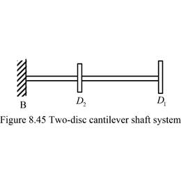
449 |
Figure 8.45 |
Free end disc D1
|
|
|||
|
|
450 |
Example 8.12 |
Update as per solution as per calculation EIl instead of EIl^3 ... Hence, EIl Update Table 8.13 |
|
|||
|
|
452 |
Exercise 8.4 |
Add in the end “Take E = 2.1 x 10¹¹ N/m2.” |
|
|||
|
|
452 |
Exercise 8.7 |
o All disc diameter to be capital D (same for
all other examples?) o Add: For a Jeffcott rotor with an offset disc, the
following influence coefficients are valid (Refer Table A.1-7 for Deflection
relations in terms of z) |
|
|||
|
|
454 |
Exercise 8.8, Line 4 |
Shaft segments, of diameter 0.01 m, have the Make disc diameters as D1, D2, … “take diameter of
discs as |
|
|||
|
|
454 |
Exercise 8.9 |
“The masses of discs are m1 = 5 kg, m2 = 2 kg,” The diametral mass moments of inertia of the discs … |
|
|||
|
|
455 |
Exercise 8.12 |
The mass of the |
|
|||
|
|
456 |
Exercise 8.16, Line 7 |
…m4 = 7 kg, and m5 = 8 kg. |
|
|||
|
|
457 |
Exercise 8.17 |
1. Consider the rotor system shown in Figure 8.63 for obtaining the transverse natural frequency 2. A thin disc, of mass 3 kg
and diametral mass moment of inertia 0.01 kg-m2, is … |
|
|||
|
|
|
Exercise 8.18 |
1. Consider the rotor system shown in Figure 8.63 for obtaining the transverse natural frequency 2. A thin disc, of mass 3 kg
and diametral mass moment of inertia 0.01 kg-m2, is … |
|
|||
|
|
458 |
Exercise 8.21 |
Exercise 8.21 Obtain the
natural frequencies of the rotor system shown in Figure 8.66. Assume the
rotor has
free–free boundary conditions. Take the shaft material Young’s
modulus as E = 2.1 × 10¹¹ N/m2.
diametral mass moments of inertia of the disc are mass and gyroscopic effects. Use the TMM |
|
|||
|
|
|
|
|
ignore |
|||
|
|
459 |
Exercise 8.27 |
Delete from the end “and the
diametrical mass moment of inertia of the disc” |
|
|||
|
|
|
|
|
|
|||
|
|
462 |
subscript |
?? |
|
|||
|
|
462 |
|
add formula for simply supported beam with a
moment at some location. https://www.engineeringtoolbox.com/beams-fixed-both-ends-support-loads-deflection-d_809.html |
|
|||
|
|
|
|
Exercise
9.10 (cantilever two disc cases) Try to uniformalise In Exercise 9.8 Take D1D2 = 50 mm (as per figure) In Exercise 8.9 Take D1D2
= 75 mm and m1 = 2 kg and m2 = 5 kg (as per Examples 8.3, 8.7 and 8.11) In Example 8.11 Take left disc as D2 (in figure) m1 (5 kg)
> m2 (2 kg) 9.2/9.10/8.2 are similar problems (in 9,10
take D1D2 = 50 mm?) |
|
|||
|
Ch09 |
468 |
Fig. 9.1 subscript |
Change all |
|
|||
|
|
492 |
[Nf] |
NF1 is multiplication of first two terms in brackets |
|
|||
|
|
499 |
Eqn. (g) |
|
|
|||
|
|
499 |
Eqn. (h) |
|
|
|||
|
|
503 |
Example 9.3 |
following natural frequencies
of the system
|
|
|||
|
|
527 |
Example 9.9 (spelling of Rayleigh’s) |
For Example 9.2 obtain the Rayleigh’s damping coefficients |
|
|||
|
|
508 |
Fig. 9.20 (Example 9.5) |
Mass at node 2 is 1 kg; also below Fig. 9.20 “m2 = 1 kg” |
|
|||
|
|
530 |
Example 9.10 (in the end) |
which gives natural frequencies as
On comparison with Example 9.2 ( |
|
|||
|
|
538 |
Exercise |
(Assume the mass density, r = 7800
kg/m3 of shaft material) |
|
|||
|
|
538 |
Exercise 9.2 |
Add in the end “The shaft is
made of steel with 2.1 x 10^11 N/m^2 as Young’s modulus, E,
and 7800 kg/m^2 as the mass density, ρ.” |
|
|||
|
|
539 |
Exercise 9.8 |
Assume the mass density, r = 7800
kg/m3 of shaft material |
|
|||
|
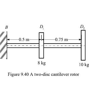
|
540 |
Exercise 9.10 |
change in fig. distance between two discs
0.75 m)
|
|
|||
|
|
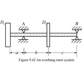
540 |
Exercise 9.12 |
b = c = 0.7 m Draw Fig. 9.42 proportionately
|
|
|||
|
|
542 |
Exercise 9.14, second line |
simply supported end conditions |
|
|||
|
|
|
|
|
|
|||
|
Ch11 |
|
||||||
|
|
613 |
Example 11.2 |
A rigid rotor of mass 5 kg |
|
|||
|
|
614 |
Table 11.2 |
Correct in 3Row 2Column as: (a3 a2
- a4 a1)
|
|
|||
|
|
624 |
Equation 11.47 |
|
✔ |
|||
|
|
633 |
Example 11.7 |
Correction in moment of area
formulae (correct all numbers accordingly) Solution: The
stiffness of the shaft in two principal directions are given as
with
and
with
Now, we have
and
Hence, the rotor will be unstable in speed range 42.47 rad/s to 47.19 rad/s due to shaft asymmetry and also in speed range of 21.23 to 23.59 rad/s due to unbalance. |
|
|||
|
|
644 |
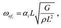
Eqn. 11.114 |
Replace
l with L
|
|
|||
|
|
645 |
Between Eqn. 11.118 and to 11.119
(first term |
which can be rearranged to
|
|
|||
|
|
645 |
Between Eqn. 11.119 up to 11.121 |
Replace
l with L
|
|
|||
|
|
667 |
Equation 11.221 |
negative sign is giving -negative imaginary part so not a physical
solution? since square of natural frequency cannot
be negative? |
|
|||
|
|
671 |
|
Herein, the moment is taken with respect to the G, the
moment can also be taken about C. In that case moment equation will contain
only theta. But since Eqns. (a) and (b) contain theta we still need to solve
all three equations simultaneously. In chapter 2 the moment was taken about
the C to get EOM in theta direction (Eqn. 2.44), page 40). |
|
|||
|
|
675 |
Exercise 11.2 |
Shift this to Exercise of chapter 10 |
|
|||
|
|
|
|
|
|
|||
|
|
676 |
Exercise 11.2 |
Add at the end “(i) Consider only stiffness direct and cross-coupled
linear coefficients. (ii) Consider both stiffness and damping direct and
cross-coupled linear coefficients.” |
|
|||
|
|
667 |
Exercise 11.8viii |
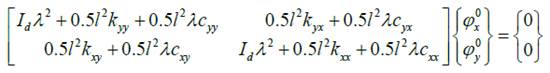
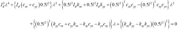
11.8 (viii) A rotor-bearing system has the following
properties: rotor mass, m = 1 kg, equivalent bearing
stiffness and damping coefficients of both bearings are kxx = kyy
= 10 kN/m, kxy = 10 kN/m, kyx = 1 kN/m, cxx = cyy = 10 kN-sec/m,
cxy = 10 kN-sec/m, cyx = 0.1 kN-sec/m |
|
|||
|
|
678 |
Exercise 11.8xxiii |
A Jeffcott rotor
with an elliptical cross-section shaft (with semi-major
axis a = 6 cm and semi-minor axis b = 4 cm). The second moment of areas about two principal axes
are given as pab3/4 and pa3b/4. The disc mass is 20 kg, the shaft span l = 1 m and Young’s modulus E = 2.1´1011N/m2. The instability zones in the rotor system due to
unbalance excitation would be within the speed range of (in rad/s) (A) 156 – 215 (B)
616.45 to 924.67 (C)
169 – 258 (D)
136 - 289 |
|
|||
|
|
678 |
Exercise 11.8xxvi |
steam whirl stiffness = 89.44 kN/m. |
|
|||
|
|
|
|
|
|
|||
|
Ch12 |
|
||||||
|
|
689 |
Below Eqn. 12.8 |
Delete as shown below:
|
|
|||
|
|
|
|
|
|
|||
|
Ch13 |
|
||||||
|
|
723 |
Example 13.4 |
Add in the end: From the construction, the
measurement will be in clockwise so residual unbalance angle =
From triangle OEA, let the
angle OAE is f2, then we
have
For residual unbalance angle = |
|
|||
|
|
729 |
Example 13.5 |
From end 7th line to be corrected as: |
|
|||
|
|
|
Example 13.5 update all data |
We have, influence coefficients as
a11 = 17.1542 +69.0116i mm/kg and a12 = 1.1199e+02 - 1.0444e+01i mm/kg It is given that machine is symmetric about the centreline, hence
Measurements, influence coefficients and correction
mass are related as
which can be simplified as
with delta = -1.6901e+04 + 4.7070e+03i which gives the balancing mass and its angular position as
wR = 0.3270 - 0.0762i kg
wR_mag = 0.3358 kg
wR_ang = -13.1223
deg.
and
wL = -0.2304 - 0.4165i kg wL_mag = 0.4760 kg wL_ang = -118.9496 deg. |
|
|||
|
|
733 |
Below eqn. 13.31, replace x with c for mode shapes |
For example, for simply supported boundary conditions, mode shapes are (i) I - mode : |
|
|||
|
|
736 |
Eqn. 13.51 (use m1n and m2n) |
|
|
|||
|
|
737 |
Equation 13.54 |
Second term has (z1):
|
|
|||
|
|
756 |
Exercise 13.2 |
Last line correct as “a
necessary correction mass required” |
|
|||
|
|
756 |
Exercise 13.5, Line 1 |
Add in the first line “…the influence coefficient method for Exercise 13.4.” |
|
|||
|
|
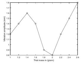
758 |
Exercise 13.12 |
Let x be
the amplitude difference with unit trial |
|
|||
|
|
758 |
Exercise 13.13 |
Exercise
13.13 In the dynamic balancing of a rigid rotor by using the influence coefficient
method, let the following measurement were made (i)
|
|
|||
|
|
758 |
Exercise 13.15 |
Exercise
13.15 In
a simply supported rotor for flexible rotor balancing |
|
|||
|
|
759 |
Exercise 13.16, Line 3 |
Delete as suggested the repeated sentence:
|
|
|||
|
Ch14 |
|
|
|
|
|||
|
|
784 |
Example 14.2 |
The horizontal load produces
displacement of 10.3 μm and
3.3 μm in the horizontal and vertical
directions respectively, |
|
|||
|
|
784 |
Example 14.3 (update numbers) |
As per solution |
|
|||
|
|
817 |
Exercise 14.6 (in end add) |
Take rotor speed equal to 2000 rpm |
|
|||
|
|
817 |
Exercise 14.7 |
by the method of unbalance excitation (all measurement are done at 100 Hz speed), the following t |
|
|||
|
|
817 |
Exercise 14.11(i) |
C) taking measurements with different
unbalance levels at a constant rotor speed |
|
|||
|
|
818 |
Exercise 14.11(vii) |
(C) when two orbits
are elliptical and identical in shape (but not in size) and
orientation. |
|
|||
|
|
|
|
|
|
|||
|
Ch15 |
825 |
Para 2 |
Line 6: Amplitudes and phases of
displacements, velocities Line 7: For
acoustics three quantities are important: level, intensity, and power. Line 9: machine these parameters
(vibrations and acoustics) and
their analyses |
|
|||
|
|
826 |
Para 2 |
For
example, an instrument (for example, in thermometer (or voltmeter)) with
a 30 cm (or 360°) scale would... |
|
|||
|
|
827 |
Example 15.1 |
1. actual
value of 1050–1000
= 50 rpm, 2.
Hence, the tachometer could be used confidently to measure speed within
± (1040
× 0.096) = ±9.62 = ±10 rpm. 3. and absolute random error from mean
of 0, 10, 10, 10 and 10 rpm |
|
|||
|
|
828 |
Frequency
range: |
the accelerometer of |
|
|||
|
|
830 |
Below Eqn.
(15.7),Line 2 |
“Equation (15.6)” |
|
|||
|
|
833 |
Above Eqn. 15.8 |
The first natural frequency of a cantilever continuous beam is expressed as (refer Table 9.2) |
|
|||
|
|
833 |
Example 15.3, last para |
compared to the uncertainty. In one parameter, then should be compared to the uncertainty in one parameter, then |
|
|||
|
|
834 |
Example 15.4 |
For L = 60 mm, from Equation 15.8, we have the Similarly, for L = 200 mm, we have the |
|
|||
|
|
841 |
-k(y2-y1) |
Eqn. + sign to be replaced by – as
|
|
|||
|
|
856 |
Example 15.11 last lines |
The output voltage is therefore E = {(3.557 /10)×10−3}(10−4 )= 3.557 ×10^−11 V should be The output voltage is therefore E = {(3.557 /10)×10−3}(10−4
)= 3.557 ×10^−8 V and reduces to approximately 2.0 × 10^5 times should be reduces to approximately 178 times |
|
|||
|
|
857 |
Exercise 15.6 |
|
|
|||
|
|
858 |
Exercise 15.8 |
z = 0.72 |
|
|||
|
|
858 |
Exercise 15.8 |
Use Y
instead of x? i.e., |
|
|||
|
|
858 |
Exercise 15.9 |
Use Y
instead of x? that |
|
|||
|
|
858 |
Exercise 15.9 |
changes
in last line "1-" to be deleted: such that |
|
|||
|
|
858 |
Exercise 15.10 |
seismic accelerometer is equal to |
|
|||
|
|
858 |
Exercise 15.13 |
|
|
|||
|
Ch16 |
887 |
Last para |
Change last but one line "to a number of multiplications of
the order of" to “to a number of multiplications to" |
|
|||
|
|
888 |
First para |
Fourth line: “which is only 2pN/N2 = 2p/N
of ...” to be changed to “so their ratio is only 2pN/N2 = 2p/N of ...” |
|
|||
|
|
924 |
Exercise 16.6xii |
Windowing operations are performed on vibration signals to (A) to
increase amplitude of main frequencies (B) reduce the leakage error (C) to
decrease amplitude of spurious frequencies (D) all
other three options |
|
|||
|
|
924 |
Exercise 16.6xvi |
D. Bisymmetrical |
|
|||
|
|
|
|
|
|
|||
|
Ch17 |
|
|
|
|
|||
|
|
978 |
Exercise 17.3 viii |
(D) 600 Hz Should be (D) 30 Hz |
|
|||
|
|
928 |
section 17.1 1st para second line |
and it is inherently inexistent. should be and it is inherently in existent. |
|
|||
|
|
935 |
|
bending moment with eight DOFs
per node. Should be bending moment with eight DOFs
per element. |
|
|||
|
|
955 |
section 17.8 second paragraph last but 2 line |
at tooth engagement, unbalance, ben shaft, worn/defective bearings, improper
backlash, and poor should be bent shaft |
|
|||
|
|
969 |
|
o TThe unbalanced sinusoidal voltage
has should be The unbalanced sinusoidal voltage has o polyphaseinduction should be polyphase induction |
|
|||
|
|
970 |
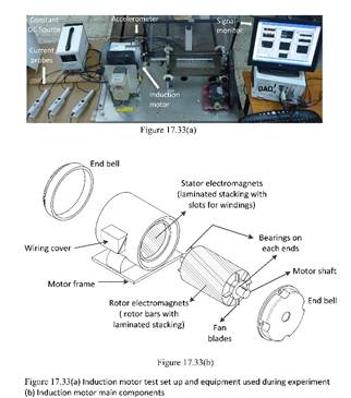
Figure 17.33 |
|
|
|||
|
|
972 |
Table 17.7 |
Short circuit freq. o
for s = 0.0375 and s = 0.0375 in Harmonics index, k may
be deleted o
81.5 Hz and
1.5 Hz (when i = 3 and n = 1), should be 81.5 Hz and 158.5 Hz (when i = 3 and n = 1), |
|
|||
|
|
|
|
|
|
|||
|
|
972 |
Table 17.7 |
o Bearing failure 76.60 Hz and 159.6 should be Bearing failure... (refer
Figure 17.39) 79.60 Hz and 159.6 o Bearing outer race fault characteristic should be Bearing outer race fault characteristic o Short circuit frequency, fst (Hz) should be Short circuit frequency, fst
(Hz) (refer Figure 17.37) o Broken bar frequency sidebands, fb should be Broken bar frequency sidebands, fb |
|
|||
|
|
972 and 974 (text) |
Table 17.7 |
o
Bearing fault case I calculated from f0 = 0.4nfr at 2341 rpm (39.02 Hz) of should be calculated from f0 = 0.4nfr at 2242.5 rpm (37.375 Hz) of o also in Table 17.7 fo = 0.4Zfr (Refer Table
17.2) at fr should be fo = 0.4Zfr (Refer Table
17.2) at fr also 0.4 × 8 × 39.02 = 119.60 Hz should be 0.4 × 8 × 37.375 = 119.60 Hz |
|
|||
|
|
973 |
|
of pole pairs, i = 1, 3, 5, . . . , and n = 1, 2, . . ., (Gandhi et al.,
2011). Change to: of pole pairs, the supply current
harmonics, i = 1, 3, 5, . . . , and the side band harmonics, n = 1, 2, . . .,
(Gandhi et al., 2011). |
|
|||
|
|
975 |
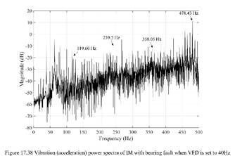
Figure 17.38 |
FIGURE
17.38 y-axis is “Magnitude” (not “Stator current’)
|
|
|||
|
|
|
|
|
|
|||
|
|
|
|
|
|
|||
|
Ch18 |
991 |
Above Figure 18.1 |
The angle is measured from the pole
pair center line, Where a is the half of the
angle subtend between a pair-pole, i.e. from the centre
line of a pair-pole to one of the pole. |
|
|||
|
|
991 |
Table 18.1 |
3-pole pairs at 45o: 0.9659 4-pole pairs at 30o and also at 60o:
1.366 |
|
|||
|
|
992 |
Eqn. (18.1) |
|
|
|||
|
|
1008 |
Fig. 18.14 |
Check for positive sign of extreme left for sensor gain? |
|
|||
|
|
1022 |
Eqn. (18.77) |
It should be corrected
as: |
|
|||
|
|
1017 |
Example 18.1 |
1. Table 18.4 Area
of core of pole-shoe magnet, 2. In Eqn. (b):
3. Eqn. (c): ki =29.0245 N/A 4. Eqn. (d): kx=7.2561´104 N/m 5. Below eqn. (a) add: Where a is the half of the
angle subtend between a pair-pole, i.e. from the centre
line of a pair-pole to one of the pole. |
|
|||
|
|
|
|
|
|
|||
|
|
1050 |
Exercise 18.1 |
Replace: amplifier gain “ |
|
|||
|
|
1050 |
Exercise 18.3(iii) |
Magnetic bearings are |
✔ |
|||
|
|
1052 |
Exercise 18.3(xix) |
Corerd as: |
|
|||
|
|
|
|
|
|
|||


|
|||||||||||||||||||||||||||||||||||||||||||||||||||||||||||||||||||||||||||||||||||||||||||||||||||||||||||||||||||||||||||||||||||||||||||||||||||||||||||||||||||||||||||||||||||||||||||