Answers

Griffiths (3.17(b))

Find the potential inside and outside a sphere shell that carries a uniform surface charge $\sigma_0$, using results of Ex. 3.9
We know the potential inside and out side must have a form

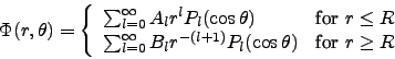$$\Phi(r,\theta)= \left\{ \begin{array}{ll} \sum_{l=0}^\inf... ...l(\cos\theta) & \mbox{for $r\ge R$\ }\\ \end{array} \right.$$ (1)

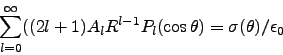
By continuity of the potential,

$$B_l = A_l R^{2l+1}$$

The normal component of the electric field is discontinuous by $\sigma/\epsilon_0$,

$$\sum_{l=0}^\infty (B_l (-l-1)R^{-l-2} - A_l l R^{l-1})P_l(\cos\theta) = -\sigma(\theta)/\epsilon_0$$

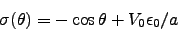
Thus,

$$\sum_{l=0}^\infty ((2l+1)A_l R^{l-1}P_l(\cos\theta) = \sigma(\theta)/\epsilon_0$$

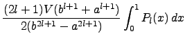
We can find $A_l$,

$$A_l = \frac{1}{2\epsilon_0 R^{l-1}} \int_0^\pi \sigma(\theta)P_l(\cos\theta)\sin\theta\,d\theta$$

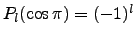
Since $\sigma$ is constant, $A_0 = R\sigma/\epsilon_0$, and is 0 for all other $l$. Then the potential is given by

$$\Phi(r,\theta)= \left\{ \begin{array}{ll} \frac{R\sigma}{... ...\epsilon_0 r} & \mbox{for $r\ge R$\ }\\ \end{array} \right.$$ (2)

Griffiths (3.18)

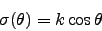
The potential at the surface of a sphere (radius $R$) is given by

$$V(\theta) = k\,\cos\,3\theta$$ (3)

where $k$ is a constant. Find the potential inside and outside the sphere, as well as the charge density $\sigma(\theta)$ on the sphere. (Assume that there is no charge inside or outside the sphere.)
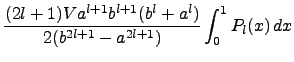
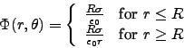
First, notice that $V(\theta)=k\cos\,3\theta=(k/5)[8 P_3(\cos\theta)-3 P_1(\cos\theta)]$. Potential is given by Eq. 1. One can find $A_l$ by comparing $\Phi(R,\theta)$ with $V(\theta)$.

$$\Phi(r,\theta)= \left\{ \begin{array}{ll} \frac{k}{5}\lef... ...ht] & \mbox{for $r\ge R$\ }\\ \end{array} \right. \nonumber$$

The charge density

$$\sigma(\theta) = -\epsilon_0 \left[ \frac{\partial\Phi}{\partial r}(R_+) - \frac{\partial\Phi}{\partial r}(R_-) \right]$$

$$= \epsilon_0 \frac{k}{5R}\left[ 56 P_3(\cos\theta) - 9 P_1(\cos\theta) \right]$$

Griffiths (3.21)

In Prob. 2.25 you found the potential on the axis of a uniformly charged disk:

$$V(r,0)=\frac{\sigma}{2\epsilon_0}(\sqrt{r^2+R^2}-r).$$ (4)

(a) Use this, together with the fact that $P_l(1)=1$, to evaluate the first three terms in the expansion (3.72) for the potential of the disk at points off the axis, assuming $r > R$. (b) Find the potential for $r < R$ by the same method, using (3.66).[Note: You must break the interior region up into two hemispheres, above and below the disk. Do not assume the coefficients $A_l$ are the same in both hemispheres.
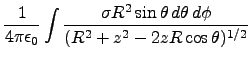
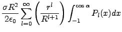
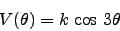
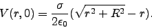
For $r > R$, on the Z-axis,

$$V(r,0)= \frac{\sigma}{2\epsilon_0}(\sqrt{r^2+R^2}-r) =\fr... ..._0} \left[ \frac{R^2}{2r} - \frac{R^4}{8r^3}+\cdots \right]$$ (5)

The Eq. 1 must match with this expression at $\theta=0$. Thus:

$$V(r,\theta)= \frac{\sigma}{2\epsilon_0}(\sqrt{r^2+R^2}-r) ... ...\cos\theta) - \frac{R^4}{8r^3}P_2(\cos\theta)+\cdots \right]$$ (6)

For $r < R$, the volume is not free of charge. Thus must be divided into two charge free regions. The expansion in terms of the Legendre polynomials will be different in different regions. In north hemisphere,

$$V(r,0)= \frac{\sigma}{2\epsilon_0}(\sqrt{r^2+R^2}-r) =\fr... ...t[ R - r + \frac{r^2}{2R} - \frac{r^4}{8R^3}+\cdots \right]$$ (7)

Thus

$$V(r,\theta)= \frac{\sigma}{2\epsilon_0}(\sqrt{r^2+R^2}-r) ... ...os\theta) - \frac{r^4}{8R^3}P_4(\cos\theta)+\cdots \right]$$ (8)

For southern hemisphere, $P_l(\cos\pi)=(-1)^l$, hence

$$V(r,\theta)= \frac{\sigma}{2\epsilon_0}(\sqrt{r^2+R^2}-r) ... ...os\theta) - \frac{r^4}{8R^3}P_4(\cos\theta)+\cdots \right]$$ (9)

Griffiths (3.37)

A conducting sphere of radius $a$, at potential $V_0$, is surrounded by a thin concentric spherical shell of radius $b$, over which someone has glued a surface charge

$$\sigma(\theta) = k \cos\theta$$ (10)

where $k$ is a constant, and $\theta$ is a usual spherical coordinate.
(a) Find potential in each region: (i) $r>b$ (ii) $a<r<b$.
(b) Find the induced charge density $\sigma_i(\theta)$ on the conductor.
(c) What is the total charge of this system? Check that your answer is consistent with the behaviour of $V$ at large $r$.
The form of potential is

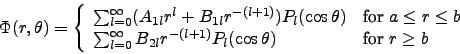$$\Phi(r,\theta)= \left\{ \begin{array}{ll} \sum_{l=0}^\inf... ... P_l(\cos\theta) & \mbox{for $r\ge b$\ } \end{array} \right.$$ (11)

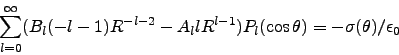
Now for each $l$, we have to determine three constants $A_{1l},B_{1l},B_{2l}$. We have three conditions of potential: (i) At $r=a$, potential is $V_0$. (ii) At $r=b$, potential must be continuous. (iii) At $r=b$, normal component of electric field must be discontinuous by $\sigma/\epsilon_0$.

$$\Phi(r,\theta)= \left\{ \begin{array}{ll} \frac{aV_0}{r}+... ...r^2} \cos\theta & \mbox{for $r\ge b$\ } \end{array} \right.$$ (12)

The charge density on the conducting surface

$$\sigma(\theta)=-\cos\theta + V_0\epsilon_0/a$$ (13)

Jackson (3.1)

Two concentric spheres have radii $a,b\,(b>a)$ and each s divided into two hemispheres by the same horizontal plane. The upper hemisphere of the inner sphere and the lower hemispheres of the outer sphere are maintained at potential $V$. The other hemispheres are at zero potential.
Determine the potential in the region $a\le r\le b$ as a series of Legendre polynomials. Include terms at least upto $l=4$. Check your solution against known results in the limiting cases $b\rightarrow\infty$ and $a\rightarrow 0$.
Begin with a general solution

$$\Phi(r,\theta)= \begin{array}{ll} \sum_{l=0}^\infty (A_{1l... ...}) P_l(\cos\theta) & \mbox{for $a\le r\le b$\ } \end{array}$$ (14)

Apply boundary conditions at both the surfaces:

$$A_l = \frac{(2l+1)V(b^{l+1}+a^{l+1})}{2(b^{2l+1}-a^{2l+1})}\int_0^1P_l(x)\,dx$$ (15)

$$B_l = \frac{(2l+1)V a^{l+1} b^{l+1}(b^{l}+a^{l})}{2(b^{2l+1}-a^{2l+1})}\int_0^1P_l(x)\,dx$$ (16)

Jackson (3.2)

A spherical surface of radius $R$ has charge uniformly distributed over its surface with a density $Q/4\pi R^2$, except for a spherical cap at the north pole, defined by a cone $\theta = \alpha$.
(a) Show that the potential inside the spherical surface can be expressed as

$$\Phi = \frac{Q}{8\pi\epsilon_0}\sum_{l=0}^\infty\frac{1}{2l... ...alpha)-P_{l-1}(\cos\alpha)]\frac{r^l}{R^{l+1}}P_l(\cos\theta)$$ (17)

where, for 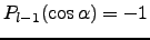$l=0$, $P_{l-1}(\cos\alpha)=-1$. What is the potential outside?
(b) What is the magnitude and the direction of the electric field at the origin?
(c) Discuss the limiting form of the potential(part a) and electric field (part b) as the spherical cap becomes (i) too small, and (ii) so large that the area with the charge on it becomes a very small cap at the south pole.
First we calculate potential at the points on the z axis.

$$\Phi(z) = \frac{1}{4\pi\epsilon_0}\int\frac{\sigma R^2\sin\theta\,d\theta\,d\phi} {(R^2+z^2-2zR\cos\theta)^{1/2}}$$ (18)

$$= \frac{\sigma R^2 }{2\epsilon_0}\sum_{l=0}^\infty \left(\frac{r^l}{R^{l+1}}\right)\int_{-1}^{\cos\alpha}P_l(x)dx$$ (19)

Since, $\int_{-1}^{\cos\alpha}P_l(x)dx = [P_{l+1}(\cos\alpha)-P_{l-1}(\cos\alpha)]/(2l+1)$ by recurrence relation. Thus,

$$\Phi(z) = \frac{Q}{8\pi\epsilon_0}\sum_{l=0}^\infty\frac{1}... ... [P_{l+1}(\cos\alpha)-P_{l-1}(\cos\alpha)]\frac{r^l}{R^{l+1}}$$ (20)

The required result is immediate.
For part b,

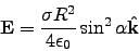$$\v{E} = \frac{\sigma R^2}{4\epsilon_0}\sin^2\alpha \v{\hat{k}}$$ (21)